(best Letterkenny voice)
Sundays are for fixin' Shiny!
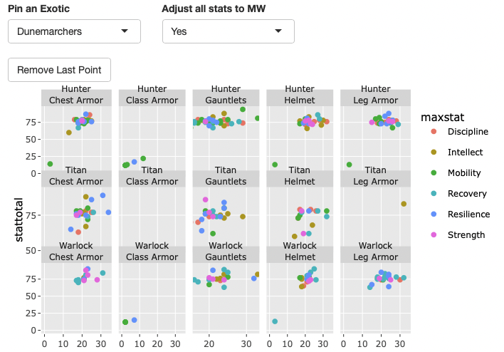
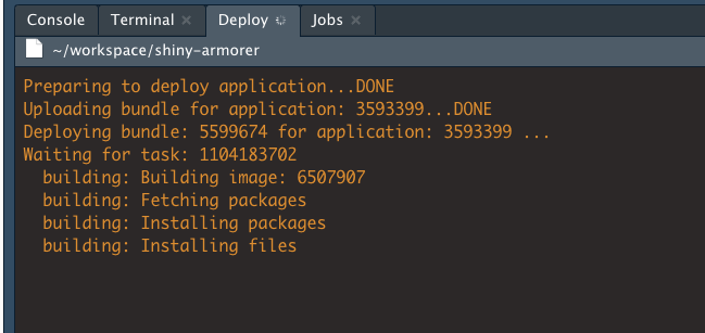
I spent a bunch of the weekend beginning a redesign of my ArmoreR project, which aims to be a Destiny 2 armor stats profiler built in R and Shiny. A year on from when I began it, I have a much better understanding of how a Shiny app works, and have also incorporated a proper, working oauth2 workflow into this revision (incorporating the things I figured out for my power level tracker). It’s really, really satisfying to be rebuilding it with all the things I’ve learned. I think the application is going to be so much better and less complicated than the first iteration. I still have a ways to go, and am happy with just how much I have transformed it with a year of learning and practice on other things.
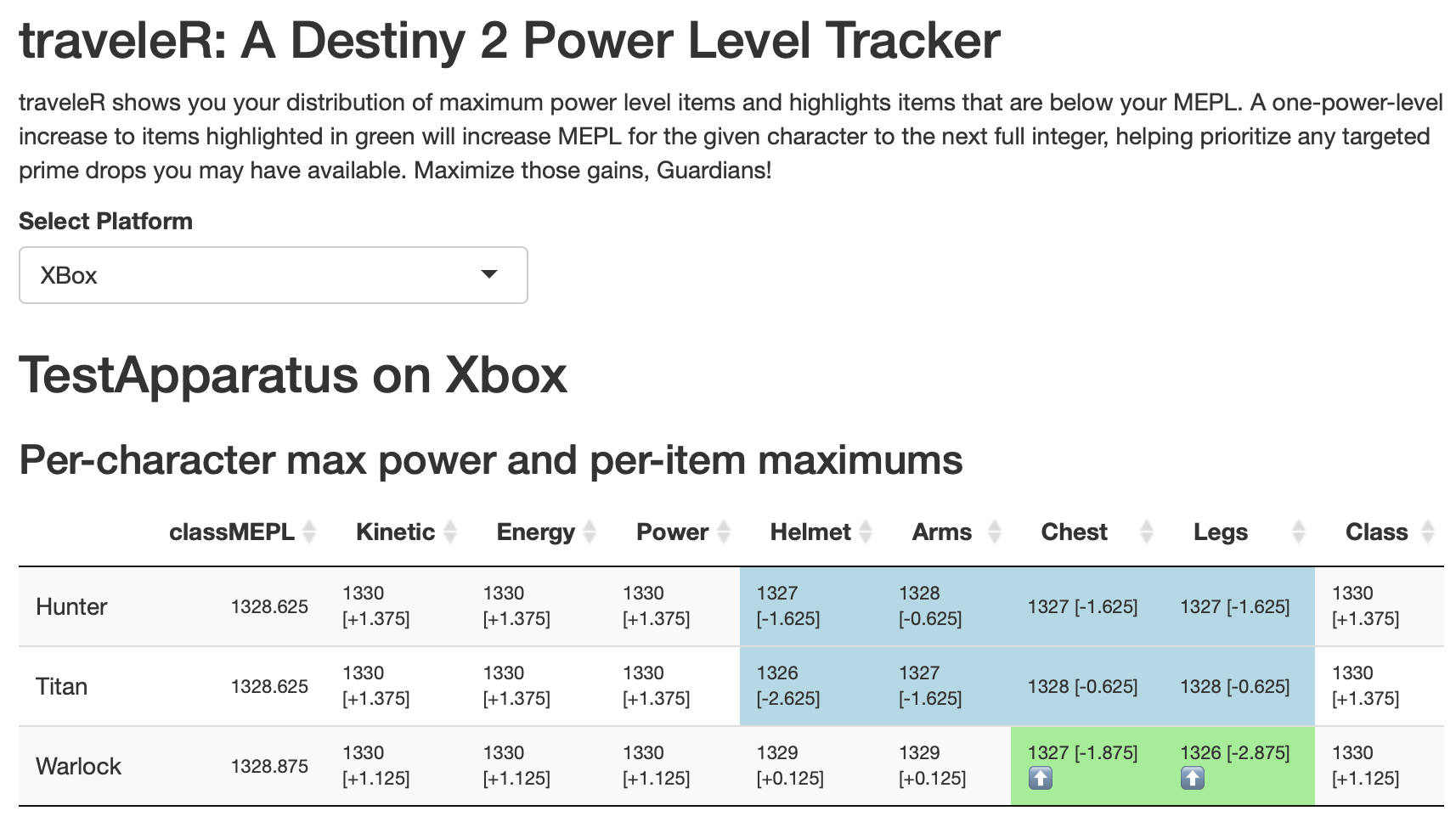
Last fall I wrote a bit about a Destiny 2 power level tracking tool I built using R. I’ve now converted it to a full-on Shiny app and solved some issues with the oauth2 flow that stumped me in my intermittent tinkering with it. I’m super satisfied to have been able to get this to work! Now that I have the authentication process figured out, I’m eager to also convert my armor profiling tool to use it. Look out!
You can check it out here: traveleR
Today I made improvements to some R code in my Destiny 2 hobby-coding-verse after learning how to much more cleanly deal with nested lists. I had previously used a solution using map() to apply a selector to each item in the list, but this was clunky, hard to remember, and became really hard to read with several levels of a nested list.
The far better solution is the unnest_auto function from {tidyr}, which I came upon when tinkering with the last.fm API data recently. Once I understood how it works, it’s so easy and satisfying! The key is to first make a named tibble.
> tibble(my_tibble = instanced)
# A tibble: 906 × 1
   my_tibble
   <named list>
 1 <named list [10]>
 2 <named list [10]>
 3 <named list [10]>
 4 <named list [10]>
 5 <named list [12]>
 6 <named list [10]>
 7 <named list [10]>
 8 <named list [10]>
 9 <named list [9]>
10 <named list [9]>
# … with 896 more rows
That nice tibble can be operated on by unnest_auto():
> tibble(my_tibble = instanced) %>% unnest_auto(my_tibble) %>%
select(itemLevel, breakerType)
Using `unnest_wider(my_tibble)`; elements have 8 names in common
# A tibble: 906 × 2
   itemLevel breakerType
       <int>       <int>
 1       132          NA
 2       133          NA
 3       133          NA
 4       132          NA
 5       133           3
 6       132          NA
 7       133          NA
 8       133          NA
 9         0          NA
10         0          NA
# … with 896 more rows
(I selected just a couple of columns for readability there; if you don’t do that, you’ll receive all fields at the current list level, including additional nested lists if they exist). After figuring this out, I realized that I also needed to keep the names of each list element, because they constitute a unique ID for the element returned from the API query, and I banged my head a bit on trying to do that as a part of the unnest operation, before I backed up, recentered on the outcome I wanted to produce, and realized I could do it really cleanly using mutate()! The final code looks like this:
> tibble(my_tibble = instanced) %>% unnest_auto(my_tibble) %>%
select(itemLevel, breakerType) %>% mutate(id = names(instanced))
Using `unnest_wider(my_tibble)`; elements have 8 names in common
# A tibble: 906 × 3
   itemLevel breakerType id
       <int>       <int> <chr>
 1       132          NA 6917529338105913753
 2       133          NA 6917529550016812142
 3       133          NA 6917529281178546429
 4       132          NA 6917529231127188610
 5       133           3 6917529301504642848
 6       132          NA 6917529234625200021
 7       133          NA 6917529193313832065
 8       133          NA 6917529182955737017
 9         0          NA 6917529417667489181
10         0          NA 6917529490520758715
# … with 896 more rows
The D2 API returns a ton of nested lists, so this simplified, accessible and effective tool is 100% getting a featured spot in my toolbox.
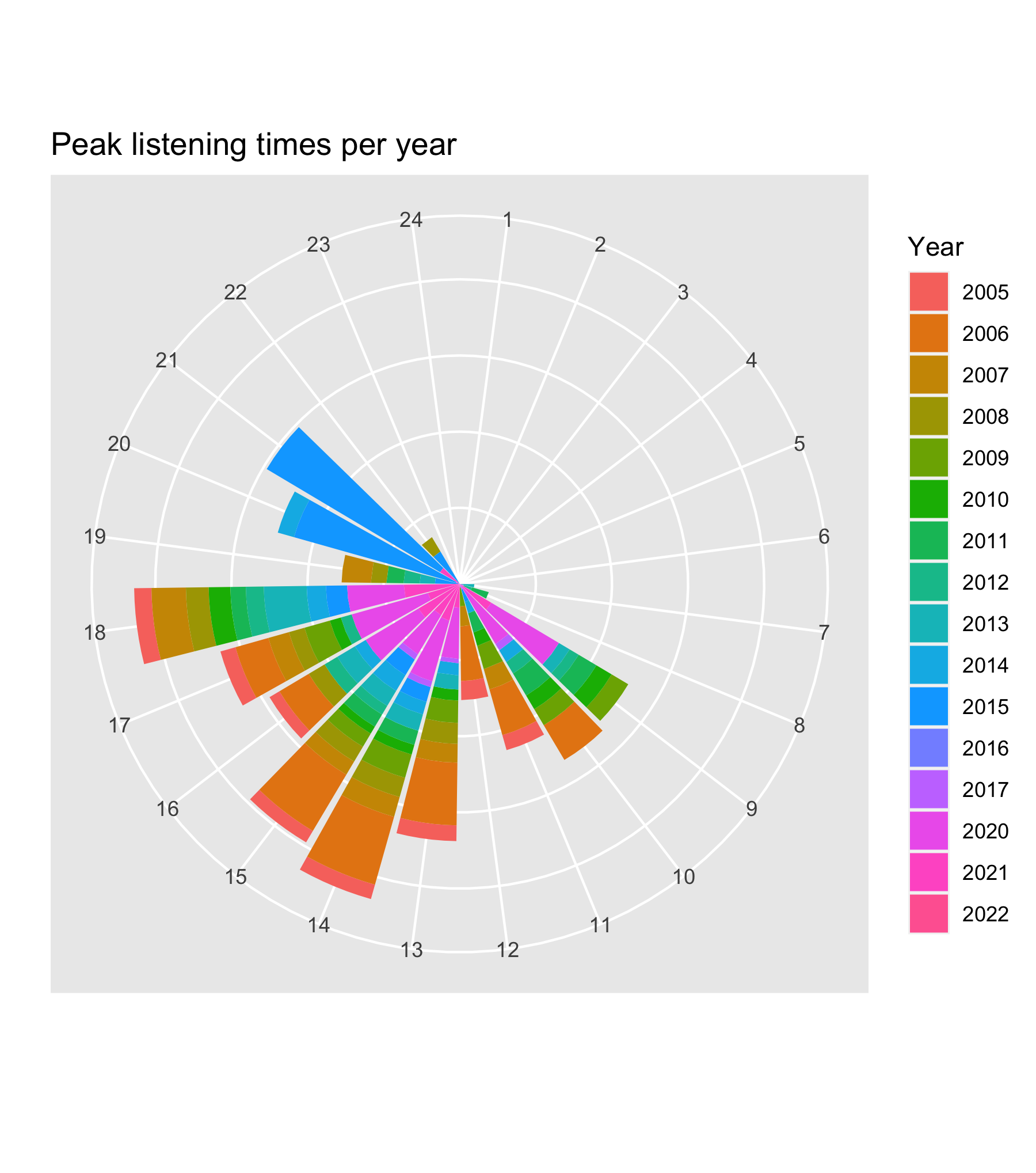
Today’s experiment with my last.fm data is this clock-like display of my peak listening hours across time. All of these would be really fun to integrate into more Shiny-based toys – maybe that will be next on my list.
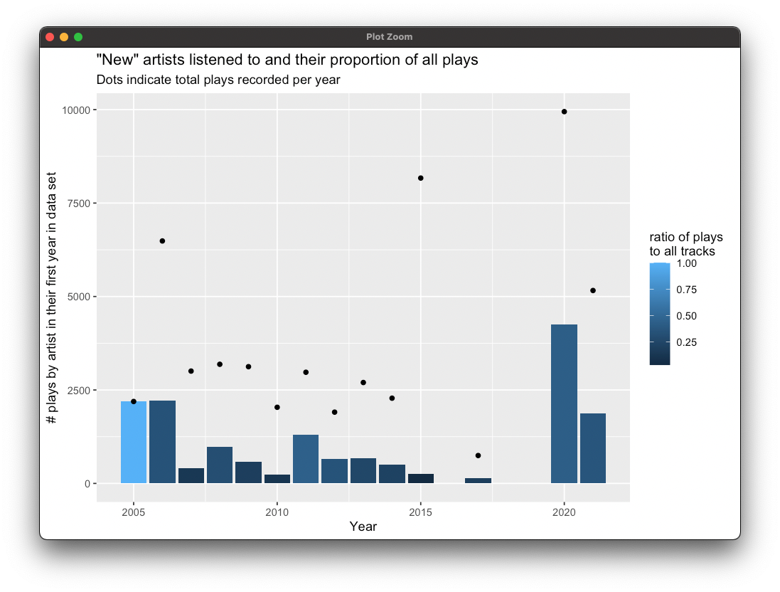
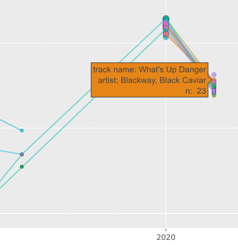
Data storytelling with last.fm: Ever since wondering if I could make something vaguely Spotify Wrapped-like with data from last.fm, I’ve dived deep into retrieving, slicing and making pictures of my music data over the past several years. Experimenting with a view of my most-played tracks over, it started to click for me just how many stories are found in this data, that this is much more than listening history – my own stories are embedded in this data, too.
In this plot of my most-played tracks for each year since 2005, you can see the huge spike in 2015, featuring huge numbers of plays of songs by Lord Huron, Frank Taylor, Hem, and Josh Ritter. I knew immediately what this was: The bedtime playlist for our kiddo, whom we would tuck in and leave to listen to songs they loved at the time. They’ve never, ever slept well without a lot of work, and for a while we had a beautiful routine of tuckins and music.

It’s a little bittersweet to see this, as it represents a really hard time in all our lives but also signifies a lot of love and, in the music itself, something that’s always been and continues to be really special.
(Methodological note: Because the spike in 2015 is so high, I had to re-do the entire plot on a log scale in order to see any variation at all in the lower-numbered tracks! I made up for that by scaling the size of the dots to the true total annual play count of each track.)
You can see the data entirely fall off a cliff after 2015. This same picture also tells the story of the death of Rdio, at one time my very favorite way to listen to music and which had great support for tools like last.fm; I replaced it with Apple Music, which has never natively supported that record-keeping, so 2015 is the last year until 2020 that I even have much of this information.
That, of course, is the first year of pandemic and also the first year I started using Roon, listening to music exclusively at home, and shifted all my workouts to home, too. So that big 2020-2021 spike of lots of colors? That’s my wife and me lifting weights and doing squat jumps in our living room!
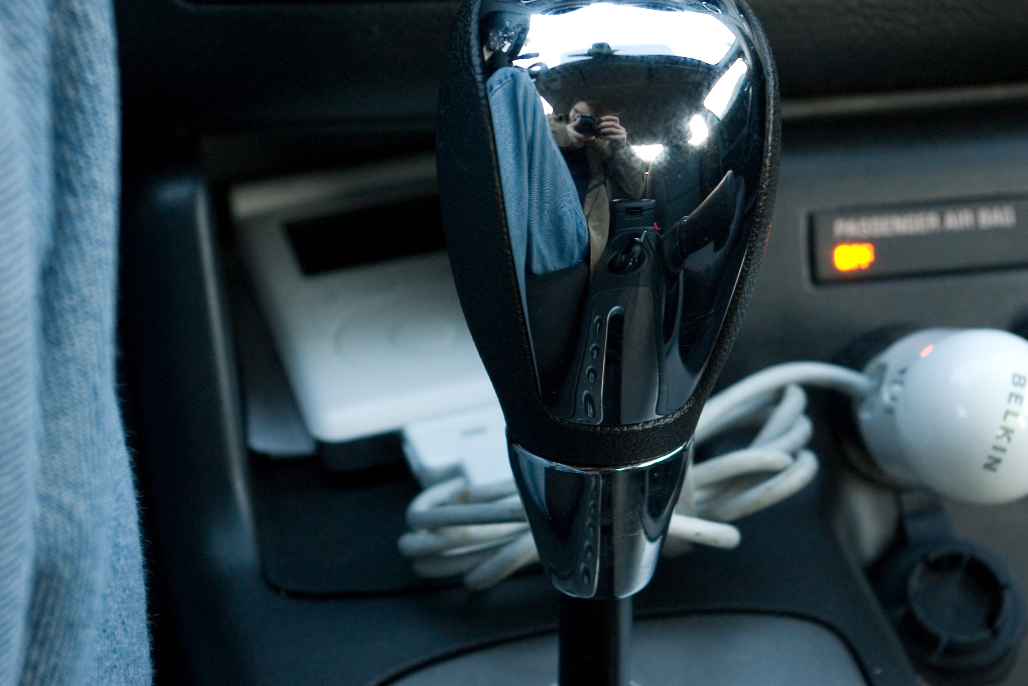
In 2007 you can see the light blue dots appear: That’s when I started listening to Josh Ritter, while away from home for a few months. I was living alone in Bellevue, WA, on a pre-doctoral internship, and carrying my iPod in my pocket while jogging or walking in the park across the street from my long-term company housing complex. I can trace those light blue dots and lines all the way through to now (though the frequency of that workout playlist swamps even my favorite artists right out of the annual top twenty). And looking at this graph I can see the trails in that little park, remember the first time I heard Josh Ritter play “Wings” in my headphones; I can recall tucking the iPod into the console of my rental car, and then spiral into memories of the post-internship vacation that my wife and I took up to the San Juan Islands, where years before I spent a summer teaching climbing.
I can click the 2011 dots to see the music I played for our kiddo in the car while driving to and from day-care. There are some silly kids songs that they used to love, and I was also on a pretty good OK Go kick at the time, so “This Too Shall Pass” was a common track in the car. God that song still gets me. I got into TV On the Radio around this time, too, and found it good car music. (Again: Thanks to Rdio, I was discovering and listening to a lot of music.)
Way back in 2005-2006 I was working at home on finishing my disseration. In iTunes I had albums from Richmond Fontaine and Tom Waits in heavy rotation – Ripped from actual CDs that I bought at Gopher Sounds in downtown Flagstaff!
I’m honestly surprised that last.fm is still operating. I’m not sure what it really does, anymore that would make revenue, but I’m glad it’s still there and that I have good tools to store my listening history once again (Oh – including now adopting Marvis as a great iOS app for scrobbling when I do listen to Apple Music again, thanks to some good discussion with music folks at micro.blog!) When scrobbling stopped working reliably there after 2015, for a while I decided that I didn’t care: listening to music was an ephemeral experience, and so would be my interest in online web-2.0 tools, I reasoned, and I made peace with leaving behind that history.
Now, as long as it continues to work, I’m so happy to have this somewhat constant and almost invisible trace, this throughline of so many moments in my life.